

(Originally written on June 1st 2023)
The researchers behind 'Deep Residual Learning for Image Recognition' aimed to address the common 'degradation problem' encountered in deep convolutional networks.
Link to paper: https://arxiv.org/pdf/1512.03385.pdf
Link to my code: https://github.com/boosungkim/Paper-Implementations
When the depth of a CNN model is increased, it initially shows an improvement in performance but eventually degrades rapidly as the training accuracy plateus or even worsens over time.
The common misconception
The common misconception is that this rapid degradation in accuracy is caused by overfitting.
While overfitting due to exploding/vanishing gradients is expected problems in very deep networks, it has been accounted for by nomalized initializations of the dataset and the intermediate Batch Normalization layers.
The degradation is definitely not caused by overfitting, as adding more layers actually causes the training error to increase.
So what causes this degradation problem? Even the researchers in the paper are not sure. Their conclusion is that "deep plain nets may have exponentially low convergence rates."
What is a Residual Learning?
So if we don't know what causes the degradation problem, do we at least know how to prevent it? That's where residual mapping in Residual Learning come into play.
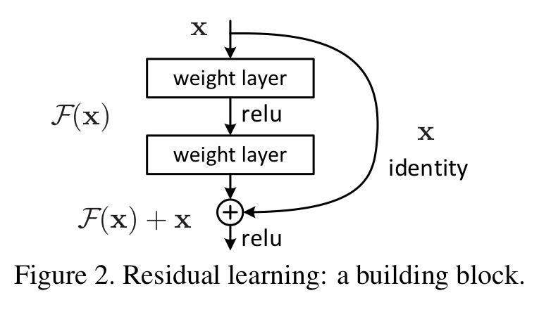
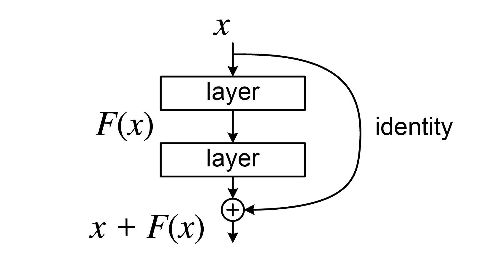
Figure 1: A residual block
If we let x be the incoming feature, the F(x) is the normal weighted layers that CNNs have (Convolutional, Batch Normalization, ReLU layers). The original x is then added (element-wise addition) to F(x) to produce H(x).
Essentially, the original features are added to the result of the weighted layers, and this whole process is one residual block. The idea is that, in the worst case scenario where F(x) produce a useless tensor filled with 0s, the identity will be added back in to pass on a useful feature to the next block. Shortcut connections can only help the network.
As this is a CNN model, downsampling is necessary. The issue is that the dimensions of F(x) and x would be different after downsampling. In such cases, the F(x) and W_1x are added together, where the square matrix W_1 is used to match dimensions.
What is a Bottleneck Residual Block?
A bottleneck residual block is a variant of the residual block that uses 1 by 1 convolutions to create a "bottleneck." The primary purpose of a bottleneck is to reduce the number for parameters in the network.
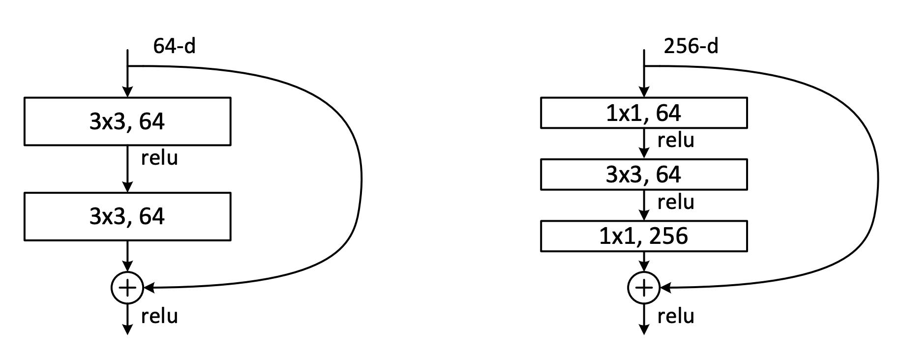
Figure 2: A no-bottleneck residual block (left) vs a bottleneck residual block (right)
By utilizing a 1x1 convolution, the network first reduces the number of channels before applying the subsequent 3x3 convolution. The output is then restored to the original channel length by another 1x1 convolution.
The reduction in the number of channels leads to a significant reduction in the number of parameters in the network. This parameter reduction allows for more efficient training and enables the use of deeper and more complex architectures while managing computational resources effectively.
Bottleneck residual blocks have become a key component in deeper ResNet variants, contributing to their improved performance and efficiency.
Understanding dimensionality reduction
As this is a CNN model, downsampling is necessary. The issue is that the dimensions of F(x) and x would be different after downsampling. In such cases, the F(x) and W_1x are added together, where the square matrix W_1 is used to match dimensions.
Below is for simple shortcut connections with elementwise addition.
z = z + identityBut what about the dimensionality reductions? Well it's just a sequence of a Conv2d layer and a BatchNorm2d layer, but matching the dimensions was a little confusing at first.
z = z + self.dim_reduction(identity)

...

def skip_connection(self, input_channels, output_channels):

return nn.Sequential(

 nn.Conv2d(in_channels=input_channels, out_channels=output_channels, kernel_size=1, stride=2, padding=0),

 nn.BatchNorm2d(output_channels)

 )
Implementation
A normal residual block
class ResidualBlockNoBottleneck(nn.Module):

 expansion = 1

def __init__(self, input_channels, output_channels, stride=1):

super(ResidualBlockNoBottleneck, self).__init__()

self.expansion = 1

self.block = nn.Sequential(

 nn.Conv2d(in_channels=input_channels, out_channels=output_channels, kernel_size=3, stride=stride, padding=1, bias=False),

 nn.BatchNorm2d(output_channels),

 nn.ReLU(),

 nn.Conv2d(in_channels=output_channels, out_channels=output_channels, kernel_size=3, stride=1, padding=1, bias=False),

 nn.BatchNorm2d(output_channels)

 )

self.relu = nn.ReLU()

if stride != 1:

self.shortcut = nn.Sequential(

 nn.Conv2d(in_channels=input_channels, out_channels=output_channels, kernel_size=1, stride=2, padding=0),

 nn.BatchNorm2d(output_channels)

 )

else:

self.shortcut = nn.Sequential()

def forward(self, x):

 z = self.block(x)

 z += self.shortcut(x)

 z = self.relu(z)

return z
In the residual block (no bottleneck), there is the standard sequence of Conv2d-BatchNorm-ReLU. The key addition here is the addition of the shortcut connection.
When there is a stride of 2 in the block, there is a change in dimensionality (width and height are reduced by 2), so the dimensionality reduction is applied.
Bottleneck residual block
class ResidualBlockBottleneck(nn.Module):

 expansion = 4

def __init__(self, input_channels, in_channels, stride=1):

super(ResidualBlockBottleneck, self).__init__()

self.block = nn.Sequential(

 nn.Conv2d(in_channels=input_channels, out_channels=in_channels, kernel_size=1, stride=1, padding=0, bias=False),

 nn.BatchNorm2d(in_channels),

 nn.ReLU(),

 nn.Conv2d(in_channels=in_channels, out_channels=in_channels, kernel_size=3, stride=stride, padding=1, bias=False),

 nn.BatchNorm2d(in_channels),

 nn.ReLU(),

 nn.Conv2d(in_channels=in_channels, out_channels=in_channels*4, kernel_size=1, stride=1, padding=0, bias=False),

 nn.BatchNorm2d(in_channels*4)

 )

self.relu = nn.ReLU()

if stride != 1 or input_channels != self.expansion*in_channels:

self.shortcut = nn.Sequential(

 nn.Conv2d(in_channels=input_channels, out_channels=in_channels*4, kernel_size=1, stride=stride, padding=0, bias=False),

 nn.BatchNorm2d(in_channels*4)

 )

else:

self.shortcut = nn.Sequential()

def forward(self, x):

 z = self.block(x)

 z += self.shortcut(x)

 z = self.relu(z)

return z
The new addition here is the 1 by 1 convolutions. Also, the code checks for stride != 1 and input_channels != self.expansion*in_channels. The second condition checks if we are repeating the same residual block or if we are moving on to the next layer.
For example, for the first layer in ResNet50, the input_channels would be 64 as a result of preliminary layers. The in_channels is 64. The first layer repeats the bottleneck block 3 times. The first time, input_channels and self.expansion*in_channels would be 64 and 4*64=256 respectively. Thus, there would be a dimensionality reduction. The second and third layers would then have input_channels and self.expansion*in_channels of 256, meaning no dimensionality reduction would be required.
With these blocks coded, making a full ResNet is as easy as stacking them on top of each other.
Conclusion
The training accuracy of my VGG implementation plateued around 93.4%. My ResNet34 CIFAR10 variant managed to reach almost 95% before plateuing, suggesting that the skip connections managed to reduce training degradation as the paper set out to do. The CIFAR10 dataset is far smaller than ImageNet - probably why we do not see as big of a difference between VGG and ResNet.
Overall, this was a good paper to implement after VGG, due to small but significant alterations to the code. Next up: DenseNet.