EfficientNet Implementation

Understanding and implementing EfficientNet

(Originally written on June 15th 2023)

Unlike previous models, EfficientNet does not introduce a novel architecture. Rather, it introduces the idea of compound scaling and a base model, EfficientNet, to test the new scaling method.

Link to paper: https://arxiv.org/abs/1905.11946

Link to my code: https://github.com/boosungkim/Paper-Implementations

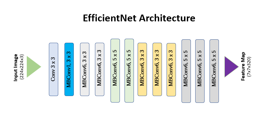
The EfficientNet utilizes inverted residual blocks from MobileNetV2, Squeeze-and-Efficient layers from SE-Net, and stochastic depth.

Scaling and balancing

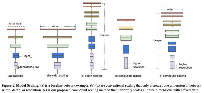
The authors argue that while scaling up depth, width, image resolution are common techniques to improve the model performance, previous papers use arbitrary scaling.

Depth is the most common method of scaling models. The VGG paper introduced the importance of depth, while ResNet and Densenet helped resolve the issue of training degradation.

While we have not spent time on width scaling, shallow networks generally use width scaling to capture features while being easy to train.

Scaling resolution is uncommon, but some networks GPipe utilize this to perform better. Resolution scaling is essentially increasing the width and height of the input images.

The empirical results of the paper indicate that a balance among width/depth/resolution can be achieved through compound scaling, which scales all three by a constant factor.

Compound scaling

The idea behind compound scaling is to uniformly scale the depth, width, and resolution of the network in a principled manner. The authors introduce a compound coefficient, denoted as φ, that controls the scaling factor for each dimension. By varying the value of φ, the network can be scaled up or down while maintaining a balance among depth, width, and resolution.

The compound scaling is achieved by applying a set of predefined scaling rules. These rules specify how the depth, width, and resolution should be scaled based on the compound coefficient φ. By following these rules, the network's capacity is increased in a balanced way, ensuring that no individual dimension dominates the scaling process.

\(\begin{align*} depth: d &= \alpha^{\phi}\\ width: w &= \beta^{\phi}\\ resolution: r &= \gamma^{\phi} \end{align*}\)

such that

\(\begin{align*} \alpha \cdot \beta^2 \cdot \gamma^2 \approx 2 \text{ and}\\ \alpha \geq 1, \beta \geq 1, \gamma \geq 1 \end{align*}\)

For EfficientNet-B0, the authors first fixed φ = 1 and performed a grid search for α, β, γ based on the equations above. The results showed that the best values are α = 1.2, β = 1.1, γ = 1.15.

Then, by fixing the α, β, γ values found above, the authors calculated new φ for scaled up versions of the model (EfficientNet-B1 ~ B7).

The authors used this approach to minimize search cost, but it is technically possible to find the optimal α, β, γ values using a larger model.

Inverted residual block (MobileNet) and SE-Net

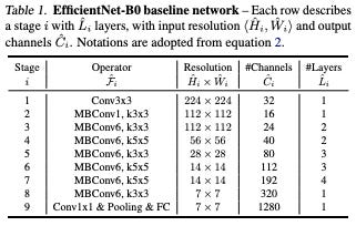
Table 1: EfficientNet-B0 architecture

As you can see from the table above, the EfficientNet-B0 baseline network utilizes inverted residual blocks (MBConv) from MobileNets.

In a normal residual block, bottlenecks are used to reduce the number of parameters and improve efficiency. To summarize, the block has a wide -> narrow -> structure using 1 by 1 convolutions.

On the other hand, an inverted residual block uses a narrow -> wide -> narrow approach with 1 by 1 convolutions and 3 by 3 depthwise convolutions.

Depthwise convolutions use far less parameters, as only one channel is neccessary for the filters. A single channel filter is used to calculate convolutions layer by layer, meaning less parameters.

The authors also state that they use Squeeze-and-Excitation networks.

Stochastic depth

Stochastic depth is essentially dropout for layers. For each mini-batch, some residual layers are completely dropped and only the residual skip connections are passed along.

This allows the network to train with a shorter effective depth, reducing the risk of overfitting and promoting regularization. By randomly dropping layers, stochastic depth provides a form of regularization similar to dropout but specifically tailored for residual networks.

SiLU

The authors of the paper use SiLU instead of ReLU for feature activation.

Conclusion

The big mistake I made was implementing this paper before MobileNet, as EfficientNet builds upon MobileNetV2. On the bright side, implementing MobileNetV2 should be relatively easy now using the code for the inverted residual block.

This is definitely the most complex model that I coded to date, as it uses many previous concepts. I haven't run this model on CIFAR10 yet, as I am still going through the code to see if I implemented everything correctly, but it was quite an experience jumping back and forth between papers and presentation videos to try and grasp the idea of EfficientNet.

Once I finalize the model and run it on a dataset, I will post another blog post.

References:

1. https://paperswithcode.com/method/inverted-residual-block